
# Example text data
texts <- c(
  "Hello world! This is an example text.",
  "Text preprocessing is essential for NLP tasks.",
  "R provides multiple tools for cleaning and analyzing text."
)

# Step 1: Create a corpus and preprocess using pipes
clean_dfm <- texts %>%
  # Convert to corpus
  corpus() %>%
  # Convert corpus to tokens (individual words)
  tokens(
    remove_punct = TRUE,   # Remove punctuation
    remove_numbers = TRUE  # Remove numbers
  ) %>%
  # Convert to lowercase
  tokens_tolower() %>%
  # Remove stopwords
  tokens_remove(stopwords("english")) %>%
  # Optional: stem words
  tokens_wordstem() %>%
  # Convert tokens to document-feature matrix (DFM)
dfm()Quantitative Text Analysis (QTA)
A very brief introduction to QTA and sentiment analysis
Research Data Services (RDS)
Workshops and more 👀

Text-as-Data Approach
Text-as-Data Approach: Example 1
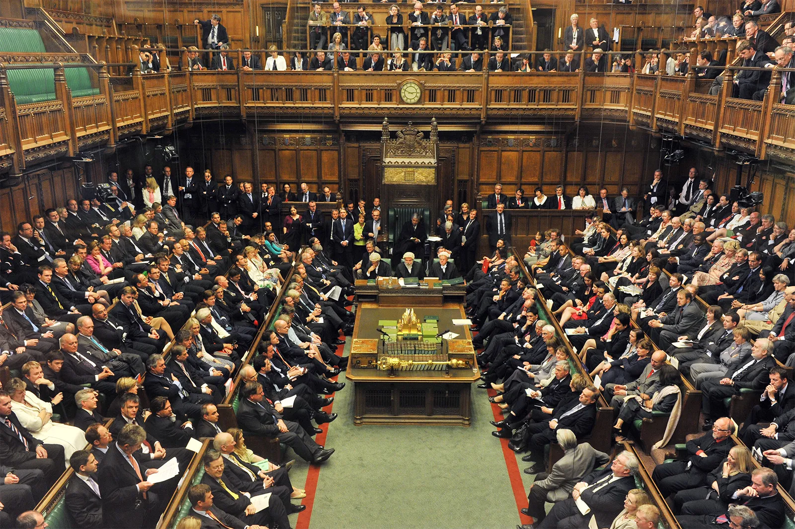
Photo Source, Parliamentary speeches are great example of big text data
Text-as-Data Approach: Example 2
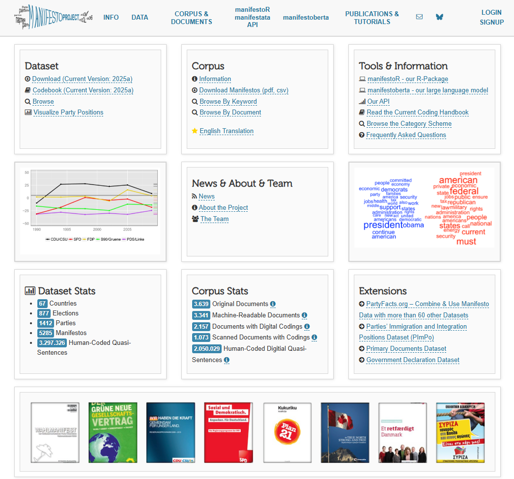
Photo Source, Manifesto Project sponsored by APSA
Text-as-Data Approach: Example 3

Photo Source, Social media is another great source of text-data
Text-as-Data Approach: Example 4
- Different applications show that Ngram data correlates strongly with similar data from well-respected sources.
- Ngrams has content validity – i.e., good proxy
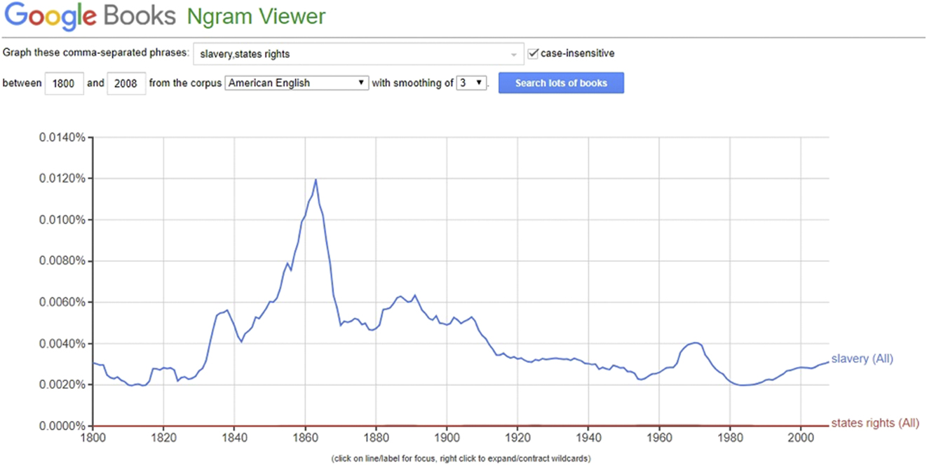
Source: Richey S, Taylor JB. Google Books Ngrams and Political Science: Two Validity Tests for a Novel Data. PS: Political Science & Politics. 2020; 53(1):72-77. doi:10.1017/S1049096519001318
Basic QTA (Quantitative Text Analysis) Process
Computers see text differently
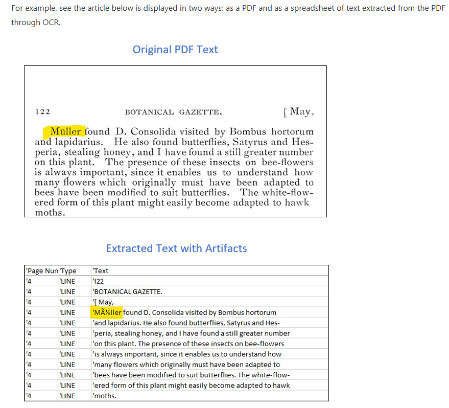
Source: https://guides.library.illinois.edu/datacleaning/textdata
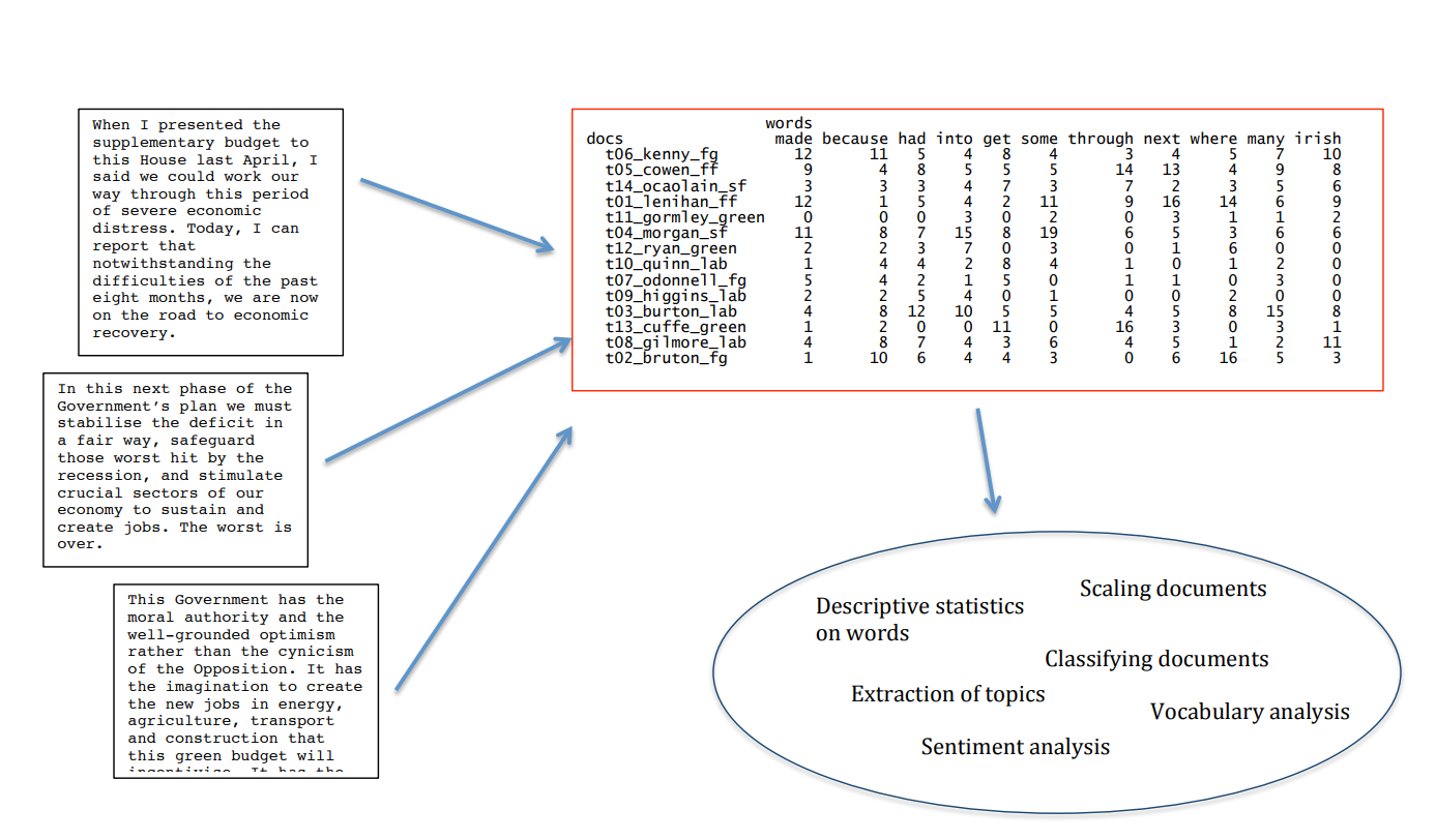
Texts → Feature matrix → Analysis
Prerequisites for QTA
- have a good understanding of quantitative methods (OLS and beyond)
- familiarity with a software … Preferably R to run your models
- (optional) ability to process text files in a programming language such as Python
- (optional but highly recommended) familiarity with regex
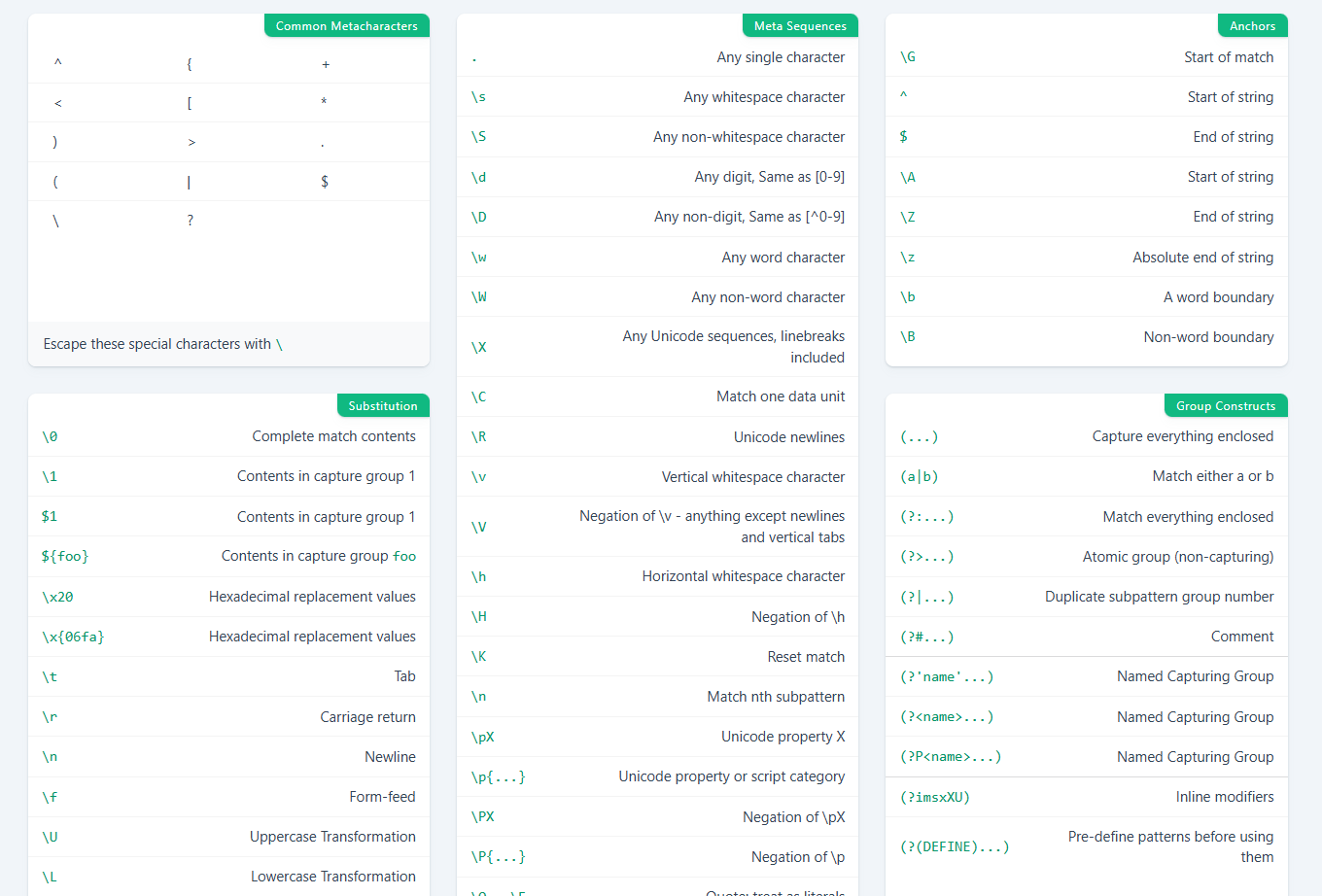
What is regex?
Regular expressions (hereafter, regex): describing patterns with strings
can test whether a string matches the expression’s pattern
can use a regex to search/replace characters in a string
very powerful, but tough to read for human eye
/[a-zA-Z_\-]+@(([a-zA-Z_\-])+\.)+[a-zA-Z]{2-4}/regex pattern to validate email addresses
It will match “user@domain.com” but not match “user@domain”
Example: words with berry
black<berry>, blue<berry>, cran<berry>, straw<berry>
In R, you can look at a whole text, and retrieve any word that has berry in it
str_view(my_data, "berry")
What is regex?
Why quantitative text analysis?
Justin Grimmer’s haystack metaphor: QTA improves reading
Analyzing a straw of hay: close reading, understanding the meaning of a sentence
- Humans are great at it! But computers struggle
Organizing the haystack: describing, classifying, scaling texts
- Humans struggle. But computers are great at it!
Principles of quantitative text analysis (Grimmer & Stewart, 2013)
All quantitative models are wrong – but some are useful
Quantitative methods for text amplify resources and augment humans
There is no globally best method for automated text analysis
Validate, validate, validate (i.e., to ensure that what is to be measured (i.e., the numerical scores assigned to texts) correspond to the true nature of the construct being studied)
Overview of text as data methods
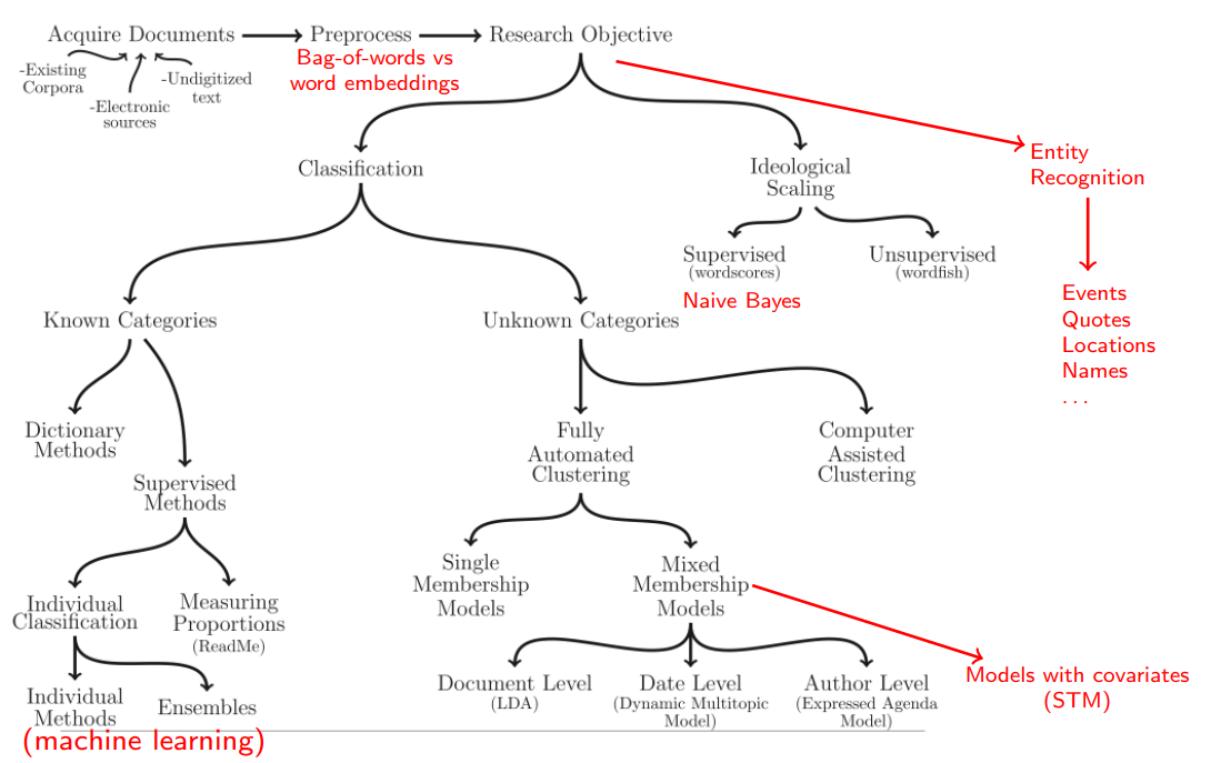
Figure 1 in Grimmer and Stewart (2013)
Ideological scaling
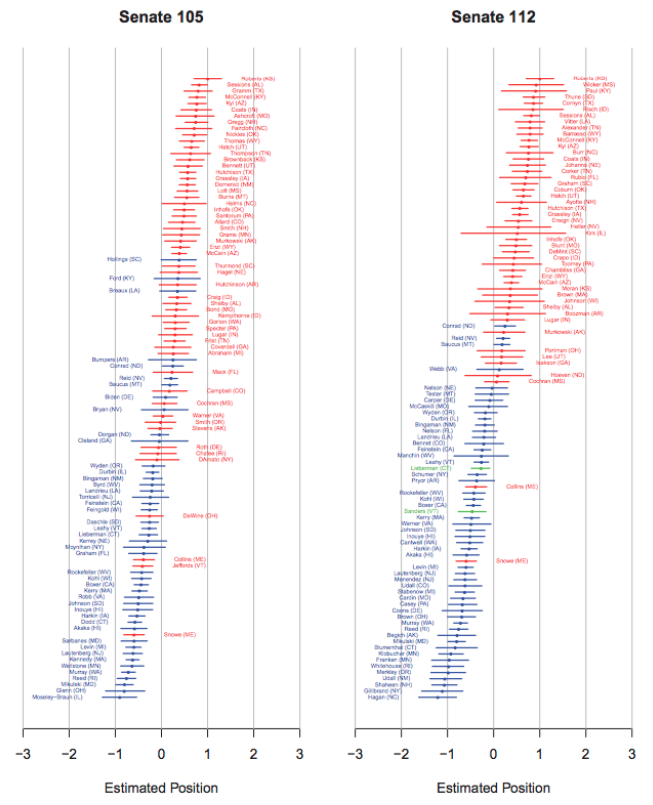
Lauderdale, B. E., & Herzog, A. (2016). Measuring political positions from legislative speech. Political Analysis, 24(3), 374-394.
Ideological scaling – explanation
- analysis of the U.S. Senate, we use all debates from January 1995 to the end of October 2014, covering the 104th to the 113th Senate
- partisan polarization of Senators apparent from the increased degree to which the scores correlate with party
- In contrast, in the 112th, there is much cleaner separation between the parties
Descriptive text analysis
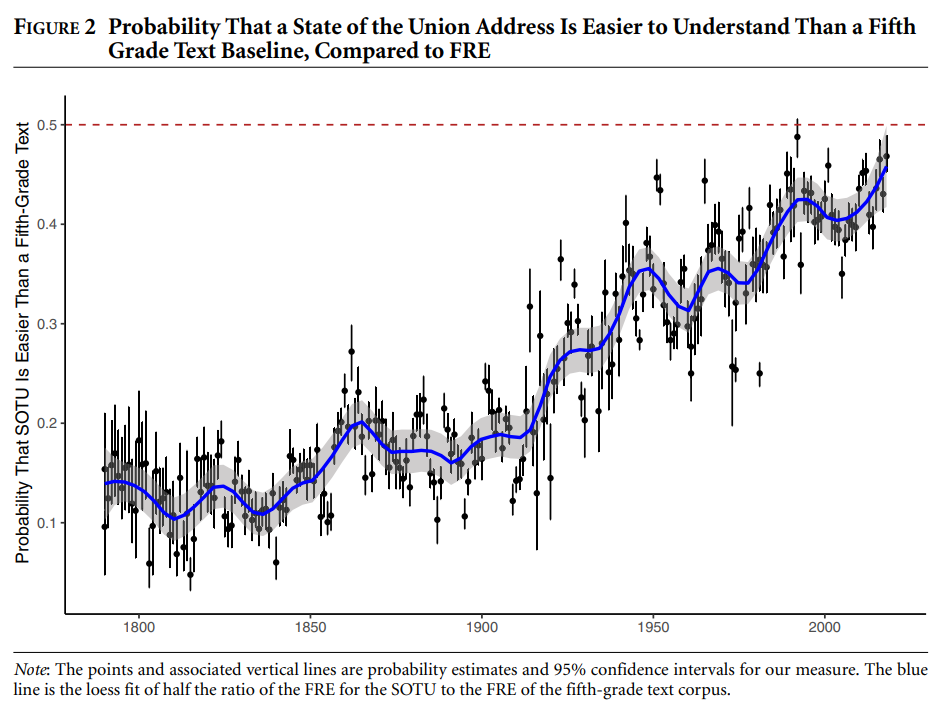
Benoit, K., Munger, K., & Spirling, A. (2019). Measuring and Explaining Political Sophistication through Textual Complexity. American Journal of Political Science, 63(2), 491–508.
Document classification into unknown categories
Bauer, Barbera et al, Political Behavior, 2016.
Data: General Social Survey (2008) in Germany
Responses to questions: Would you please tell me what you associate with the term “left”? and would you please tell me what you associate with the term “right”?
Open-ended questions minimize priming and potential interviewer effects
Automated text analysis to discover unknown categories and classify responses
Document classification into unknown categories
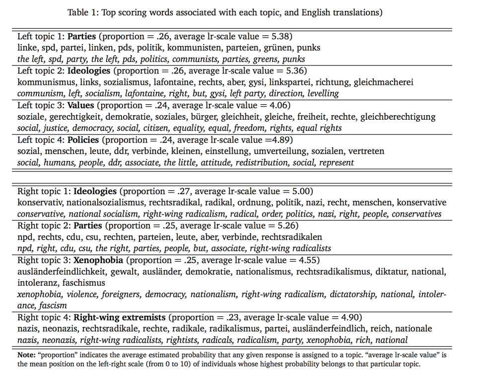
Bauer, P. C., Barberá, P., Ackermann, K., & Venetz, A. (2017). Is the left-right scale a valid measure of ideology? Individual-level variation in associations with “left” and “right” and left-right self-placement. Political Behavior, 39(3), 553-583.
Document classification into unknown categories
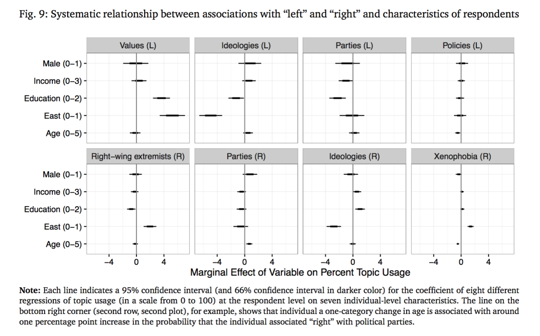
Bauer, P. C., Barberá, P., Ackermann, K., & Venetz, A. (2017). Is the left-right scale a valid measure of ideology? Individual-level variation in associations with “left” and “right” and left-right self-placement. Political Behavior, 39(3), 553-583.
Quantitative text analysis requires assumptions
Texts represent an observable implication of some underlying characteristic of interest
An attribute of the author
A sentiment or emotion
Salience of a political issue
Texts can be represented through extracting their features
most common is the bag of words assumption
many other possible definitions of “features” (e.g. word embeddings)
A document-feature matrix can be analyzed using quantitative methods to produce meaningful and valid estimates of the underlying characteristic of interest
Key feature of quantitative text analysis
- Selecting texts: Defining the corpus
- Conversion of texts into a common electronic format
- Defining documents: deciding what will be the documentary unit of analysis
Key feature of quantitative text analysis (cont.)
- Defining features: These can take a variety of forms, including tokens, equivalence classes of tokens (dictionaries), selected phrases, human-coded segments (of possibly variable length), linguistic features, and more.
- Conversion of textual features into a quantitative matrix
- A quantitative or statistical procedure to extract information from the quantitative matrix
- Summary and interpretation of the quantitative results
Some key basic concepts
- (text) corpus a large and structured set of texts for analysis
- document each of the units of the corpus
- tokens any word – so token count is total words
e.g. A corpus is a set of documents. A corpus can be 2 documents, where each document is a sentence. The first document has 7 tokens. The second has 8 tokens. (We ignore punctuation for now.)
stems words with suffixes removed (using set of rules, i.e., playing is play)
lemmas canonical word form (the base form of a word that has the same meaning even when different suffixes or prefixes are attached)
word: win winning wins won winner
stem: win win win won winner
lemma: win win win win win
“key” words Words selected because of special attributes, meanings, or rates of occurrence
stop words Words that are designated for exclusion from any analysis of a text
Preprocessing text
Preprocessing helps us to go from words to numbers:
Preprocess text: lowercase, remove stopwords and punctuation, stem, tokenize into unigrams and bigrams (bag-of-words assumption)
Preprocessing text in R
Preprocessing text in R
Document-feature matrix of: 3 documents, 14 features (61.90% sparse) and 0 docvars.
       features
docs    hello world exampl text preprocess essenti nlp task r provid
  text1     1     1      1    1          0       0   0    0 0      0
  text2     0     0      0    1          1       1   1    1 0      0
  text3     0     0      0    1          0       0   0    0 1      1
[ reached max_nfeat ... 4 more features ]
# Step 2: Optional - get top features/words
top_words <- textstat_frequency(clean_dfm) %>%
head(10) # Top 10 most frequent words
print(top_words) feature frequency rank docfreq group
1 text 3 1 3 all
2 hello 1 2 1 all
3 world 1 2 1 all
4 exampl 1 2 1 all
5 preprocess 1 2 1 all
6 essenti 1 2 1 all
7 nlp 1 2 1 all
8 task 1 2 1 all
9 r 1 2 1 all
10 provid 1 2 1 allWord frequencies and their properties
Bag-of-words approach disregards grammar and word order and uses word frequencies as features. Why?
Context is often uninformative, conditional on presence of words
Individual word usage tends to be associated with a particular degree of affect, position, etc. without regard to context of word usage
Common English stop words
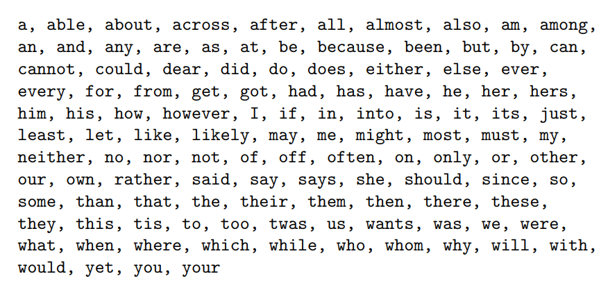
But no list should be considered universal! Also, not all languages are the same!
Where to get text data?
Some tips…
- Existing datasets, e.g. UCD’s EuroParl project Hansard Archive of parliamentary debates in UK Media archives (newspaper articles, TV transcripts…) at LexisNexis, ProQuest, Factiva… Academic articles (JSTOR Data for Research) Open-ended responses to survey questions
- Collect your own data: From social media (Twitter, FB) and blogs Scraping other websites
- Digitize your own text data using OCR (optical character recognition) software Use AI to improve digital texts into machine-readible version options: Tesseract (open-source), Abbyy FineReader
Your experience (ideas) with text data?
- What type of textual data have you worked with?
- What data would you be interested in collecting?
Packages and Sources for QTA in R

Source: https://www.tidytextmining.com/
Text-as-Data Approach: ``The book’’

Source: https://press.princeton.edu/books/paperback/9780691207551/text-as-data
Packages and Sources for QTA in R
- quanteda: https://quanteda.io/ and https://tutorials.quanteda.io/
- tidytext: https://juliasilge.github.io/tidytext/
- tm: https://cran.r-project.org/web/packages/tm/index.html
- textdata: https://cran.r-project.org/web/packages/textdata/readme/README.html
- UPenn’s library guide: https://guides.library.upenn.edu/penntdm/r
- Chris Bail’s course: https://cbail.github.io/textasdata/Text_as_Data.html
- sentimentr: https://github.com/trinker/sentimentr
Sentiment Analysis
- Sentiment analysis (also known as opinion mining) is a natural language processing (NLP) technique used to determine the emotional tone behind a body of text.
- It classifies text as: Positive, Negative, Neutral
- More advanced systems can detect emotions (e.g., joy, anger, sadness) or intensity (e.g., mildly positive vs. strongly positive).
Process in a nutshell
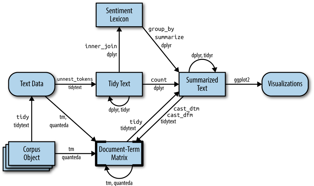
Source: https://www.tidytextmining.com/dtm
Sentiment Analysis Examples
- sentimentr package using Presidential debates
- quanteda approach using Trump vs Clinton tweets
sentimentr package – basic functions
# library(dplyr)
# library(sentimentr)

# Sample text
text <- "This workshop is awesome but the instructor is boring!"
text2 <- "This workshop is awesome. But, the instructor is boring!"

# The main function is sentiment
sentiment(text)
Key: <element_id, sentence_id>
element_id sentence_id word_count sentiment
<int> <int> <int> <num>
1: 1 1 9 -0.4498 element_id sentence_id word_count emotion_type emotion_count
<int> <int> <int> <fctr> <int>
1: 1 1 9 anticipation 1
2: 1 1 9 trust 1
3: 1 1 9 anger 0
4: 1 1 9 anger_negated 0
5: 1 1 9 anticipation_negated 0
6: 1 1 9 disgust 0
7: 1 1 9 disgust_negated 0
8: 1 1 9 fear 0
9: 1 1 9 fear_negated 0
10: 1 1 9 joy 0
11: 1 1 9 joy_negated 0
12: 1 1 9 sadness 0
13: 1 1 9 sadness_negated 0
14: 1 1 9 surprise 0
15: 1 1 9 surprise_negated 0
16: 1 1 9 trust_negated 0
emotion
<num>
1: 0.1111111
2: 0.1111111
3: 0.0000000
4: 0.0000000
5: 0.0000000
6: 0.0000000
7: 0.0000000
8: 0.0000000
9: 0.0000000
10: 0.0000000
11: 0.0000000
12: 0.0000000
13: 0.0000000
14: 0.0000000
15: 0.0000000
16: 0.0000000 element_id sentence_id word_count profanity_count profanity
<int> <int> <int> <int> <num>
1: 1 1 9 0 0sentimentr package – basic functions
# library(dplyr)
# library(sentimentr)

# Sample text
text2 <- "This workshop is awesome. But, the instructor is boring!"

# The main function is sentiment
sentiment(text2)
Key: <element_id, sentence_id>
element_id sentence_id word_count sentiment
<int> <int> <int> <num>
1: 1 1 4 0.3000000
2: 1 2 5 -0.2683282Key: <element_id>
element_id word_count sd ave_sentiment
<int> <int> <num> <num>
1: 1 9 0.4018687 0.01583592sentimentr package – Presidential debates
# Let's use the presidential debate data in sentimentr
debates <- presidential_debates_2012

# Let's create positive, negative, and neutral sentiments
debates_with_pol <- debates |> get_sentences() |> sentiment() |>
  mutate(polarity_level = ifelse(sentiment < 0.2, "Negative",
                                 ifelse(sentiment > 0.2, "Positive","Neutral")))

# Let's check negative sentences
debates_with_pol |> filter(polarity_level == "Negative") |> head()
person tot time role
<fctr> <char> <fctr> <fctr>
1: ROMNEY 2.1 time 1 candidate
2: ROMNEY 2.2 time 1 candidate
3: LEHRER 3.1 time 1 moderator
4: ROMNEY 4.1 time 1 candidate
5: ROMNEY 4.2 time 1 candidate
6: ROMNEY 4.4 time 1 candidate
dialogue
<get_sentences>
1: What I support is no change for current retirees and near retirees to Medicare.
2: And the president supports taking dollar seven hundred sixteen billion out of that program.
3: And what about the vouchers?
4: So that's that's number one.
5: Number two is for people coming along that are young, what I do to make sure that we can keep Medicare in place for them is to allow them either to choose the current Medicare program or a private plan.
6: They get to choose and they'll have at least two plans that will be entirely at no cost to them.
element_id sentence_id word_count sentiment polarity_level
<int> <int> <int> <num> <char>
1: 3 1 14 -0.1336306 Negative
2: 4 1 14 0.1336306 Negative
3: 5 1 5 0.0000000 Negative
4: 6 1 5 0.0000000 Negative
5: 7 1 40 0.1343968 Negative
6: 9 1 20 0.0000000 Negativesentimentr package – Presidential debates
# Let's look at candidates' sentiments
debates |>
  get_sentences() |>
  sentiment() |>
  ggplot() +
  geom_boxplot(aes(y = person, x = sentiment))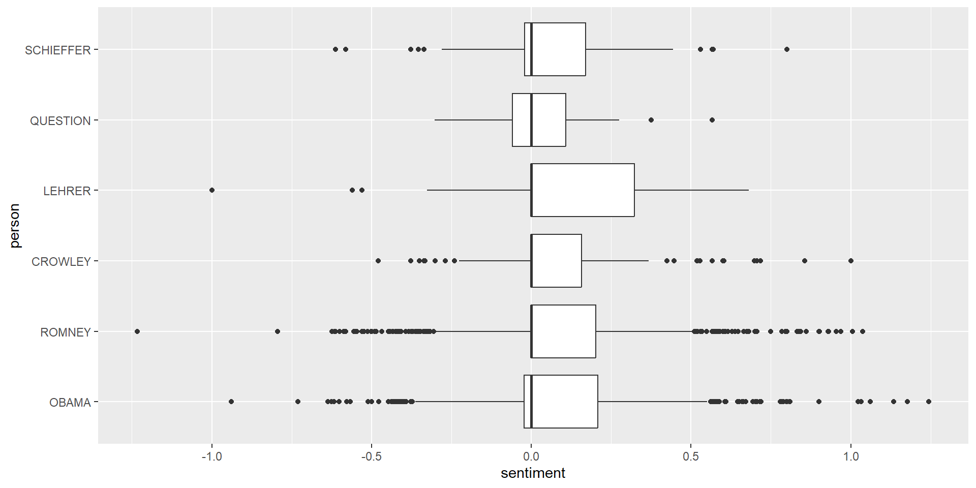
# My expectation is that overall presidential debates are neutral
debates |>
  get_sentences() |>
  sentiment_by(by = NULL)  |> #View()
  ggplot() + geom_density(aes(ave_sentiment))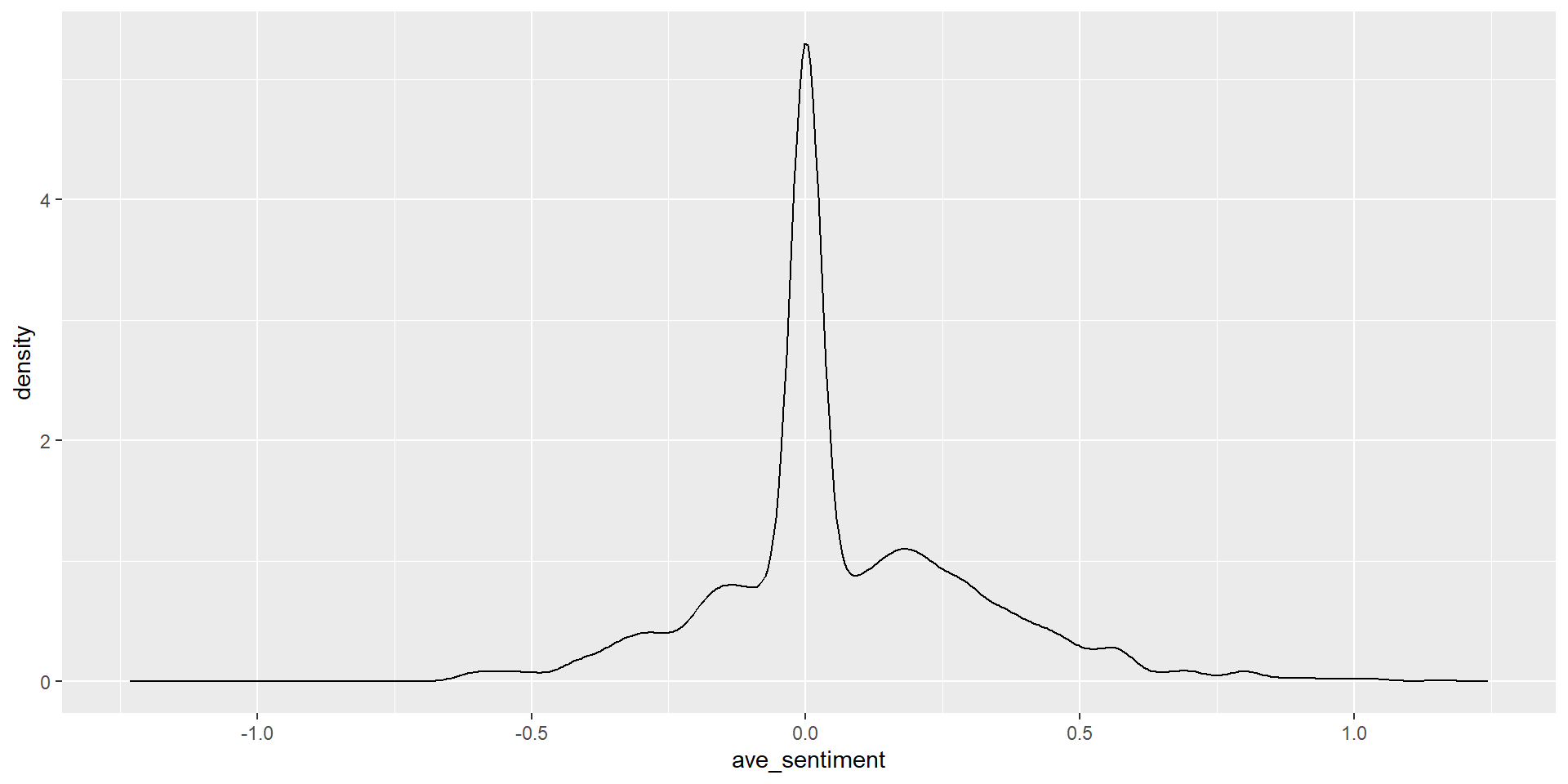
Trump vs Clinton Example – Let’s start by loading packages and data
Trump vs Clinton: Who tweets the most?
ggplot(trumpclinton.stats.monthly, aes(as.Date(paste(Year, Month, "01", sep = "-")), Tweets, group = Candidate, col = Candidate)) +
  geom_line(size = 1) +
  scale_colour_brewer(palette = "Set1") +
  scale_x_date(date_breaks = "2 months", date_labels = "%b %Y") +
  theme(axis.text.x = element_text(angle = 45, hjust = 1), legend.position = "bottom") +
  ggtitle("Trump vs. Clinton: Tweets per month (2015-2017)") +
  xlab("")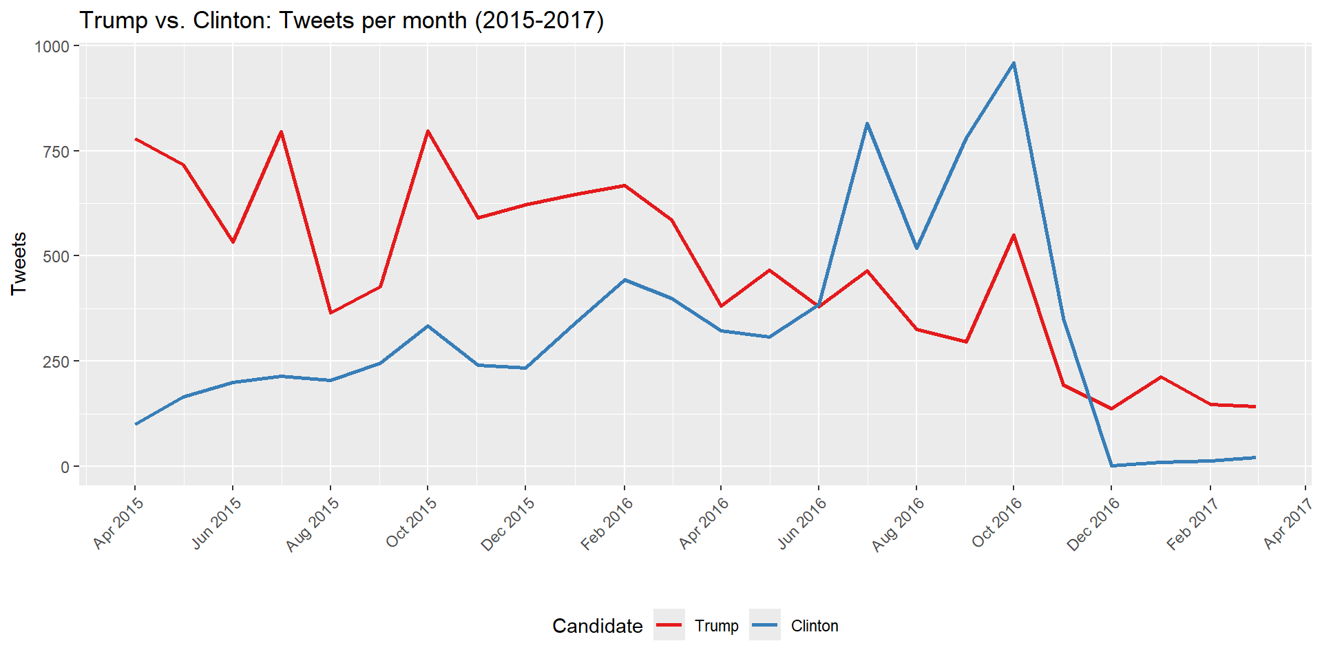
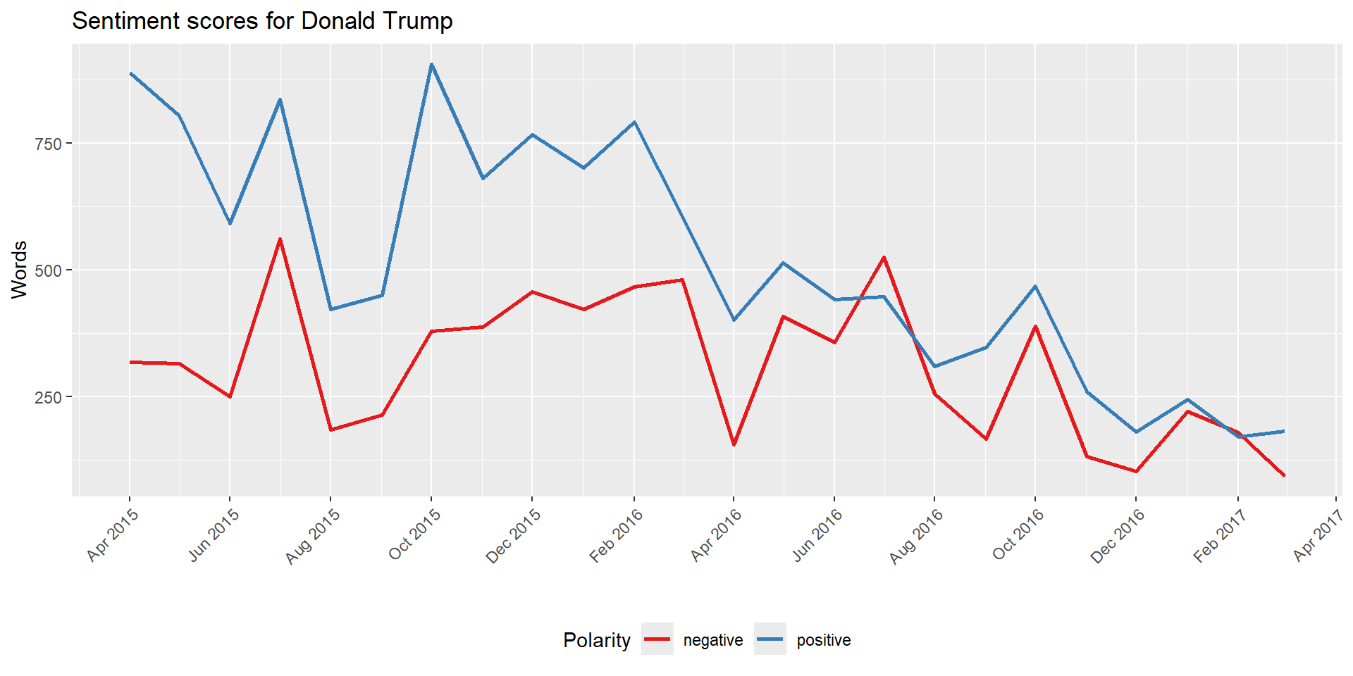
Overall sentiment in Trump’s tweets
# Create corpus specific to Trump
corpus.trump <- corpus_subset(trumpclinton.corpus, Candidate == "Trump")

# Combine Month and Year into one docvar
docvars(corpus.trump, "document") <- paste0(docvars(corpus.trump, "Month"), ".", docvars(corpus.trump, "Year"))

# Step 1: Create dfm without grouping
dfm.trump.raw <- dfm(tokens(corpus.trump))

# Step 2: Group dfm by your new 'document' variable
dfm.trump.grouped <- dfm_group(dfm.trump.raw, groups = docvars(corpus.trump, "document"))

# Step 3: Apply sentiment dictionary
dfm.trump.sentiment <- dfm_lookup(dfm.trump.grouped,
                                  dictionary = data_dictionary_LSD2015)

# Step 4: Convert to tidy format
sentiment.trump <- convert(dfm.trump.sentiment, "data.frame") %>%
  pivot_longer(cols = c(positive, negative),
               names_to = "Polarity", values_to = "Words") %>%
  mutate(Date = as.Date(paste("01", doc_id, sep = "."), "%d.%m.%Y")) %>%
  filter(Date >= "2015-04-01" & Date <= "2017-04-01")

# Step 5: Plot
trump_sentiment_plot <- ggplot(sentiment.trump, aes(Date, Words, color = Polarity, group = Polarity)) +
  geom_line(size = 1) +
  scale_colour_brewer(palette = "Set1") +
  scale_x_date(date_breaks = "2 months", date_labels = "%b %Y") +
  ggtitle("Sentiment scores for Donald Trump") +
  theme(axis.text.x = element_text(angle = 45, hjust = 1), legend.position = "bottom") +
  xlab("")
How it looks like
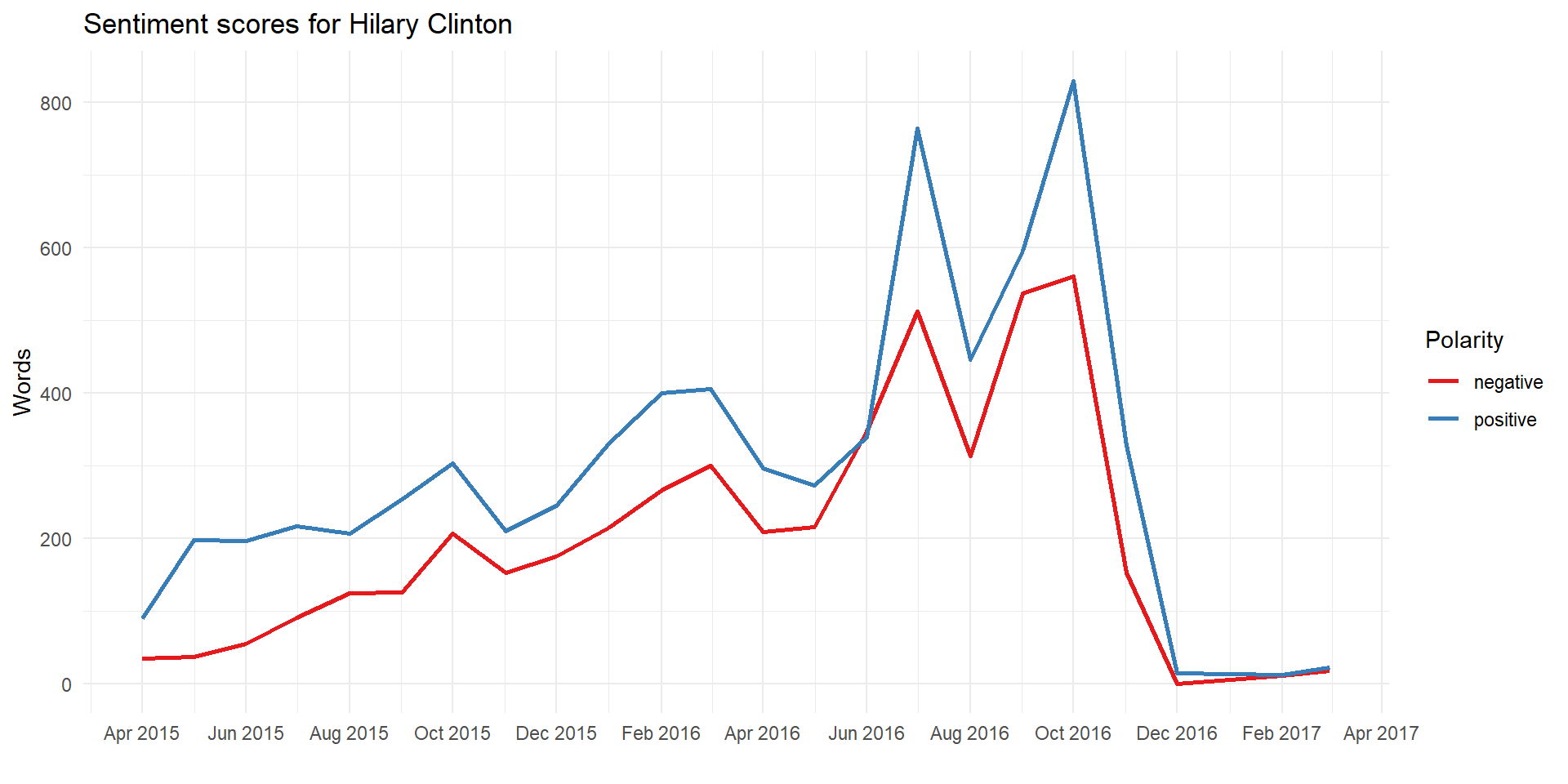
Overall sentiment in Clinton’s tweets
# Create corpus specific to Clinton
corpus.trump <- corpus_subset(trumpclinton.corpus, Candidate == "Clinton")

# Combine Month and Year into one docvar
docvars(corpus.trump, "document") <- paste0(docvars(corpus.trump, "Month"), ".", docvars(corpus.trump, "Year"))

# Step 1: Create dfm without grouping
dfm.trump.raw <- dfm(tokens(corpus.trump))

# Step 2: Group dfm by your new 'document' variable
dfm.trump.grouped <- dfm_group(dfm.trump.raw, groups = docvars(corpus.trump, "document"))

# Step 3: Apply sentiment dictionary
dfm.clinton.sentiment <- dfm_lookup(dfm.trump.grouped, dictionary = data_dictionary_LSD2015)

# Step 4: Convert to tidy format
sentiment.clinton <- convert(dfm.clinton.sentiment, "data.frame") %>%
  pivot_longer(cols = c(positive, negative),
               names_to = "Polarity", values_to = "Words") %>%
  mutate(Date = as.Date(paste("01", doc_id, sep = "."), "%d.%m.%Y")) %>%
  filter(Date >= "2015-04-01" & Date <= "2017-04-01")

# Step 5: Plot
clinton_sentiment_plot <- ggplot(sentiment.clinton,
                                 aes(Date, Words, color = Polarity, group = Polarity)) +
  geom_line(size = 1) +
  scale_colour_brewer(palette = "Set1") +
  scale_x_date(date_breaks = "2 months", date_labels = "%b %Y") +
  ggtitle("Sentiment scores for Hilary Clinton") +
  theme(axis.text.x = element_text(angle = 45, hjust = 1), legend.position = "bottom") +
  theme_minimal() +
  xlab("")
How it looks like?
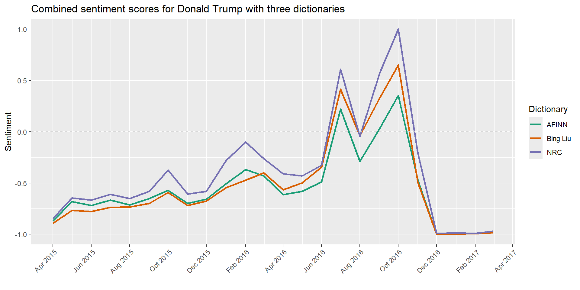
How about using different dictionaries? Comparison of AFINN, Bing Lou, and NRC dictionaries
sentiment.dictionary.bingliu <- dictionary(list(
  positive = scan("dictionaries/bingliu/positive-words.txt", what = "char", sep = "\n", skip = 35, quiet = T),
  negative = scan("dictionaries/bingliu/negative-words.txt", what = "char", sep = "\n", skip = 35, quiet = T))
  )

sentiment.dictionary.nrc <- dictionary(list(
  positive = scan("dictionaries/nrc/pos.txt", what = "char", sep = "\n", quiet = T),
  negative = scan("dictionaries/nrc/neg.txt", what = "char", sep = "\n", quiet = T)))

afinn <- read.csv("dictionaries/AFINN-111.txt", header = F, sep = "\t", stringsAsFactors = F)

sentiment.dictionary.afinn <- dictionary(list(positive = afinn$V1[afinn$V2>0],
                                              negative = afinn$V1[afinn$V2<0]))
Using different dictionaries
# Step 0: Combine Month and Year into a single docvar for grouping
docvars(corpus.trump, "document") <- paste0(docvars(corpus.trump, "Month"), ".", docvars(corpus.trump, "Year"))

# Step 1: Create plain dfm
dfm.trump.raw <- dfm(tokens(corpus.trump))

# Step 2: Group by document
dfm.trump.grouped <- dfm_group(dfm.trump.raw, groups = docvars(corpus.trump, "document"))

# Step 3: Apply different dictionaries
dfm.trump.bingliu <- dfm_lookup(dfm.trump.grouped, dictionary = sentiment.dictionary.bingliu)
dfm.trump.nrc     <- dfm_lookup(dfm.trump.grouped, dictionary = sentiment.dictionary.nrc)
dfm.trump.afinn   <- dfm_lookup(dfm.trump.grouped, dictionary = sentiment.dictionary.afinn)

# Step 4 (optional): Weight the dfm
dfm.trump.bingliu <- dfm_weight(dfm.trump.bingliu)
dfm.trump.nrc     <- dfm_weight(dfm.trump.nrc)
dfm.trump.afinn   <- dfm_weight(dfm.trump.afinn)

# Step 5: Organize in tidy format for plotting
sentiment.trump.bingliu <- convert(dfm.trump.bingliu, "data.frame") %>% mutate(Dictionary = "Bing Liu")
sentiment.trump.nrc <- convert(dfm.trump.nrc, "data.frame") %>% mutate(Dictionary = "NRC")
sentiment.trump.afinn <- convert(dfm.trump.afinn, "data.frame") %>% mutate(Dictionary = "AFINN")

# Step 6: Plot the comparison of Trump with different dictionaries
sentiment.trump.combined <- bind_rows(sentiment.trump.bingliu, sentiment.trump.nrc, sentiment.trump.afinn) %>%
  gather(positive, negative, key = "Polarity", value = "Sentiment") %>%
  filter(Polarity == "positive") %>%
  mutate(Date = as.Date(paste("01", doc_id, sep = "."), "%d.%m.%Y")) %>%
  filter(Date >= "2015-04-01" & Date <= "2017-03-01") %>%
  mutate(Sentiment = rescale(Sentiment, to = c(-1,1))) %>%
  select(Date, Dictionary, Sentiment)

trump_dictionaries <- ggplot(sentiment.trump.combined,
       aes(Date, Sentiment, colour = Dictionary, group = Dictionary)) +
  geom_line(size = 1) +
  scale_colour_brewer(palette = "Dark2") +
  geom_hline(yintercept = 0, linetype = "dashed", color = "lightgray") +
  scale_x_date(date_breaks = "2 months", date_labels = "%b %Y") +
  ggtitle("Combined sentiment scores for Donald Trump with three dictionaries") +
  xlab("") +
  theme(axis.text.x = element_text(angle = 45, hjust = 1))
How it looks like?
Conclusion – How to realistically learn QTA (Quantitative Text Analysis)?
- Make sure you have a good background in OLS and GLM
- Taking a course helps! (or training like ICPSR)
- A lot of online and free courses exists
- Work on a project that involves text-as-data